
Tutorial: Building A Basic Budget In Excel (For The Absolute Excel Beginners) Part 2
This website may earn commissions from purchases made through links in this post. As an Amazon Associate, I earn from qualifying purchases.

This tutorial is a follow on from Part One where we designed a basic budget. In this tutorial, we’ll copy and paste the budget format over to create a spreadsheet for actual income and expenses and a variation spreadsheet that will show the difference between what we budget and what we actually earn/spend.
If you haven’t already, check out Part One of this tutorial.
Click on the pictures to enlarge them. If there is anything I haven’t explained well or you have any questions please don’t hesitate to contact me either in the comments below or by email.
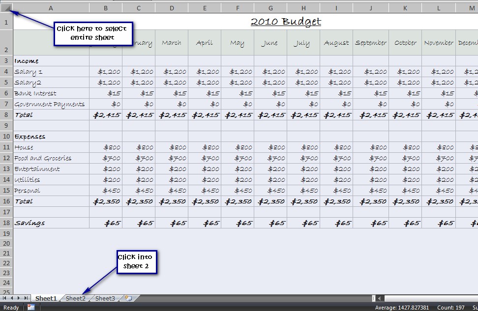
1. Select your budget using the top left button between row 1 and column A. Copy your spreadsheet, click the sheet 2 tab and click into the cell A1 and paste the budget. Paste it again into the A1 cell on sheet 3 also.
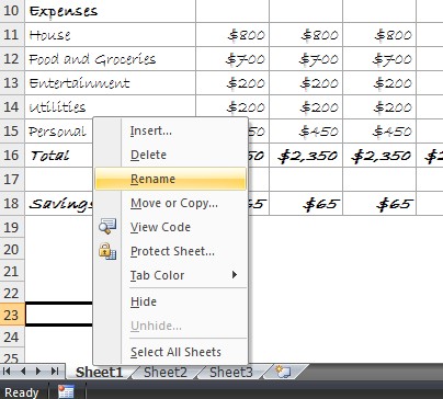
2. Right click on Sheet 1 and select Rename from the menu. Rename the tab Budget. Do the same for Sheet 2 and rename it Actual and rename Sheet 3 Variance.
3. In the Actual tab, replace the values with 0, making sure to leave the formulas intact and rename the spreadsheet 2010 Actual or something similar.
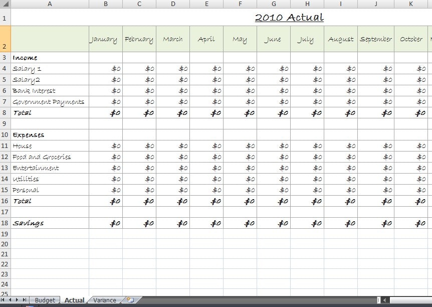
This sheet is where you enter all of your actual expenses. Use a tracking method to track actual expenses and enter them here. The totals will show what you actually earned in a month, what you actually spent and where, and your actual savings for the month. Of course, your sheet will be much more detailed than the one I’ve created as an example, but you get the idea.
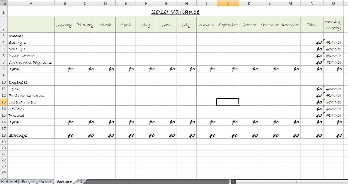
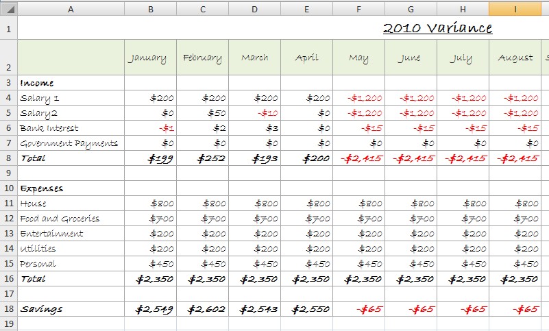
4. In the Variance tab, rename the spreadsheet 2010 Variance and delete all the values leaving the formulas intact.
This is the fun part. We’re going to use a referential formula so that once we set up the formulas in this sheet, you won’t ever have to add data, it will come across automatically.
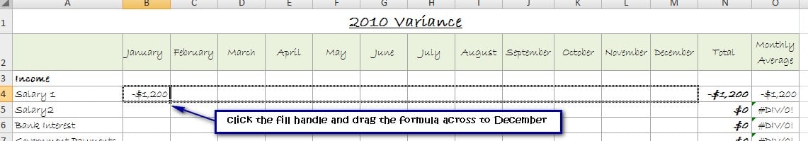
In cell B4 type = (equals sign) then click on the Actual Tab and then click on B4. Type in – (minus sign), click on the Budget tab and then click on B4. Press enter.
Your formula should look like this:
=Actual!B4-Budget!B4
(change the cell references (B4 etc) if your budget is different)
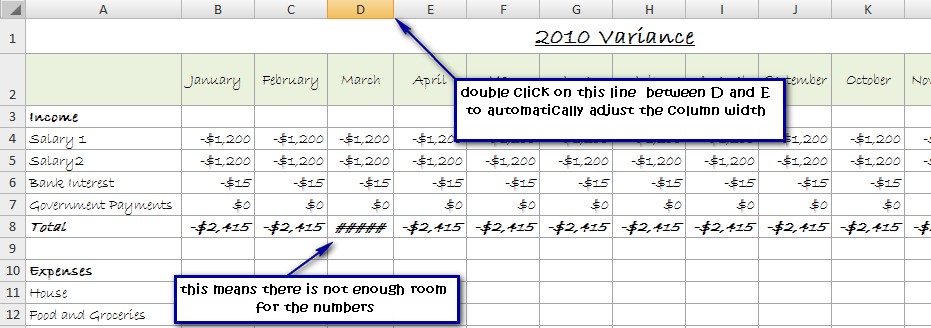
Use the fill handle to drag the formula across the row to December. Double click in the formulas to check them. Press ESC to get out of the formula. If #### comes up, just adjust the column width so that the numbers fit.
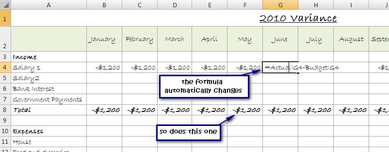
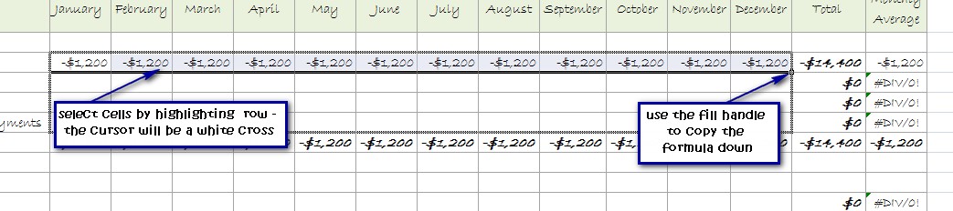
Now select the top row from January (B4) to December (M4) and using the fill handle again, drag the formula down into the rows below.
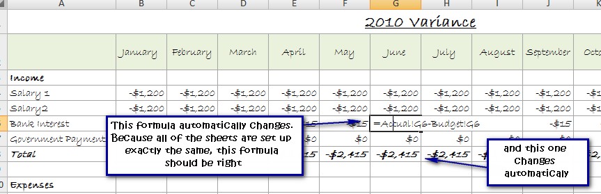
What does this show? It shows how much you actually earned for the month, less how much you budgeted. A negative number means that you earned less than you predicted, a positive number means you earned more. And it shows exactly how much more or less you earned than what you budgeted for.
5. Follow step 4 to insert a referential formula into the expenses part of the variance sheet with a slight variation, this time type:
=Budget!B11-ActualB11
(adjust the cell references to suit your budget set up)
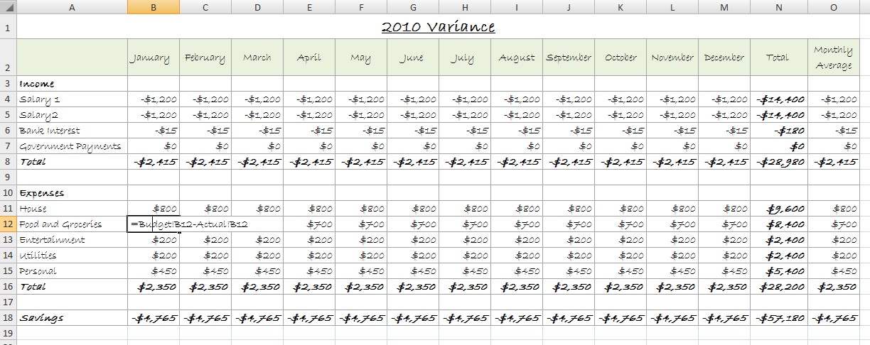
What does this show? It shows how much you budgeted to spend for the month less how much you actually spent. A negative number means that you spent more than you predicted in your budget. A positive number means that you spent less than you predicted in your budget.
Use this sheet to make judgements such as: “I only have $20 left to spend on groceries this month,” or “I overspent on going out, so I’ll have to cut down on my clothes budget this month to meet budget” etc.
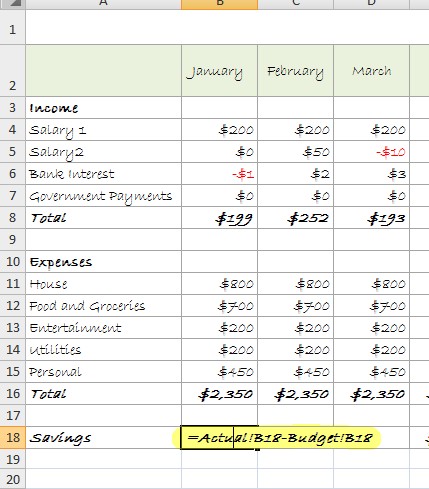
6. Change the Savings row to a referential formula (as above – Actual – budget) and fill across:
7. Test your formulas. Type some numbers into your Actual worksheet. How does it affect your Variance worksheet? Change your budget. How does that affect your Variance worksheet?
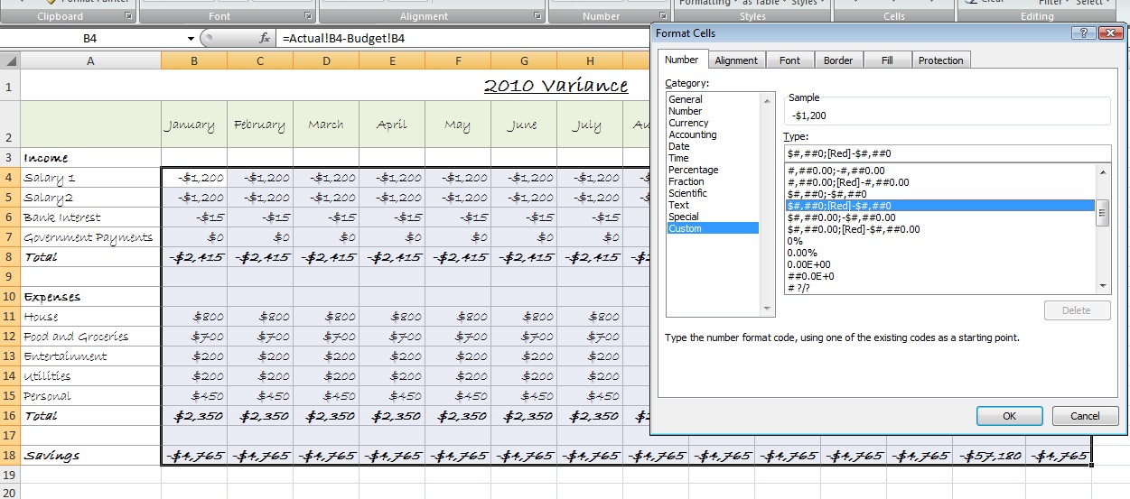
(Tip: I think that having a negative number in red helps to understand the spreadsheet at a glance. To do this select all the cells with numbers in them and go to the Number formatting section on the ribbon (Format:cell in the older versions) and select a Custom number to show negatives in red (see pic).
And that’s it for building a basic budget. Now you just need to keep it up to date by entering in your actual expenses on a regular basis.
There aren’t really any more formulas or functions that are needed to get a whole lot of data from your budget. From this basic set up, you can make your budget as detailed and complicated as you like.
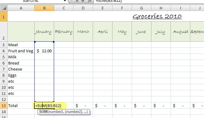
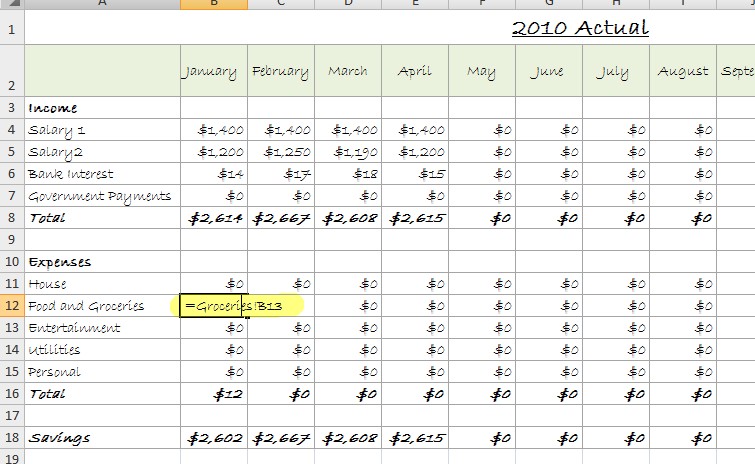
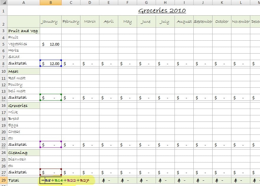
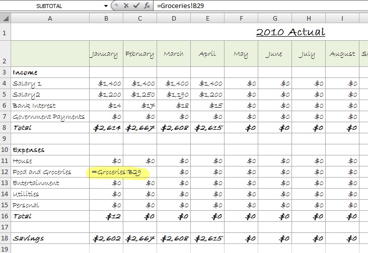
For example, I like to break up my grocery spending so I know exactly how much I spend on bread as opposed to milk etc. To do this just create another sheet for your grocery spending, add up the totals and use a referential formula to insert the totals into your Actual spreadsheet so that it updates automatically.
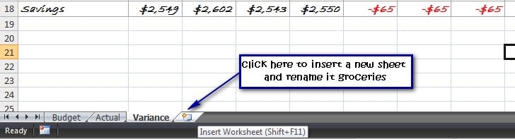
You can do this for any income or expense category and you can make it as detailed and complicated as you like:
Check out the tutorial for creating graphs in Excel in order to visualise your data. Or create a loan amortisation table in Excel to calculate loan repayments and link them into your budget.


Thankyou so much. With your help I have built my first ever excel workbook budget and I am all set to turn around my relationship with money in 2011.
I am so greatful for your step by step help.
Hi Angela,
Thank you for taking the time to comment. I’m glad this has been helpful. Any questions don’t hesitate to ask. :) Good luck with 2011.
What a fabulous step by step guide to creating your own budget. I’ve printed off the notes and now will get started in creating our own family budget. I will let you know how it goes. I’m very excited!
Hi Robyn, thanks. I would love to hear how you go!