Calculate Loan Repayments Using Excel and See How Different Scenarios will Affect Your Budget

Be empowered to make good financial decisions by using Excel. Calculate Loan Repayments using Excel and then connect your calculations to your budget to run different financial scenarios and see how each one affects your budget and your cash flow.

Check out the PMT tutorial before starting this one to create the initial data table.

Of course, making loan calculations can be done easily using free online loan calculators, but that’s not as fun as doing it yourself in Excel and this way you can link your information into your budget to run some dynamic financial scenarios.

Create Your Own Amortization Table in Excel

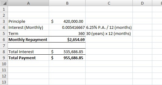
I’ll start with the same information from the PMT exercise, so if you haven’t done principal and interest calculations, do those first.

All results are based on the assumption that the interest rate remains fixed throughout the entire loan term and that interest is calculated monthly and payments made monthly. It does not take into account bank fees.

Disclaimer: This tutorial is for informational purposes only and does not constitute as professional advice. You should double-check your results with your bank or professional financial advisor. Always check with a professional financial advisor before making financial decisions.

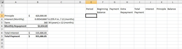
Then we’ll add some headings for the amortisation table.

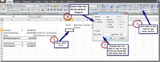
As the repayments are monthly and there are 360 months over the term of the loan, we’ll be entering the numbers 1 – 360 down the column. Use the fill – series button to complete the column quickly.

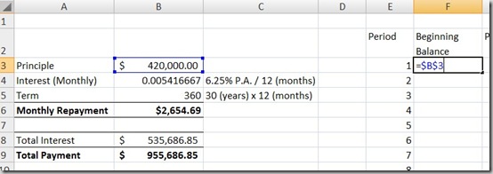
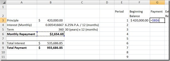
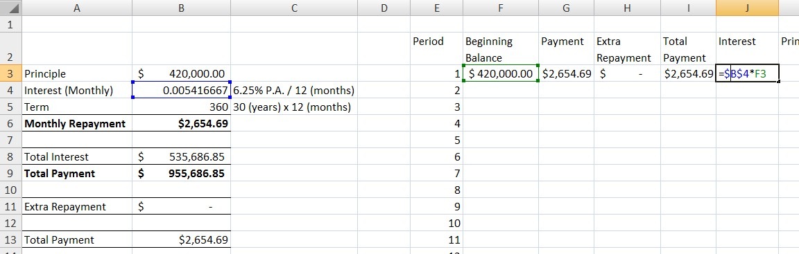
The beginning balance in the first row (period 1) is the same as the principal amount.

We’ll use a formula to put that amount into our table so if we choose to change the principal amount later on, then our whole table and results will change automatically. The dollar signs in the cell reference make it absolute: it locks in the principal amount so that it won’t move. Use the F4 key to insert the dollar signs into your formula automatically.

We’ll use the same formula for the payment amount.

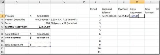
We will add an extra line under our data to show the extra repayments, and use the same formula in our table to link to this amount. For the moment I’ll leave it as $0.

And then total payment is a simple addition formula.

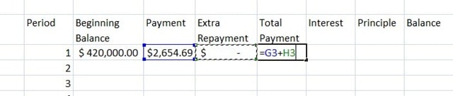
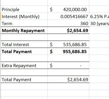
We can also summarise this total payment amount using an addition formula under our data so that we can link this to our budget later on.

To calculate the interest amount for the month, we need to multiply the monthly interest rate by the beginning balance at the start of the month. So that we can fill our formulas down, we will need to lock in the cell reference for the interest rate in our formula using the F4 key to insert dollar signs into our reference, making it absolute.

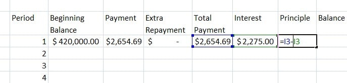
To calculate the principle portion of the monthly repayment, subtract the interest amount from the total payment amount.

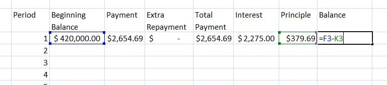
The ending balance is just a matter of subtracting the principle amount from the balance at the beginning of the month, as it’s only the principle portion of our repayment that comes off the loan balance.

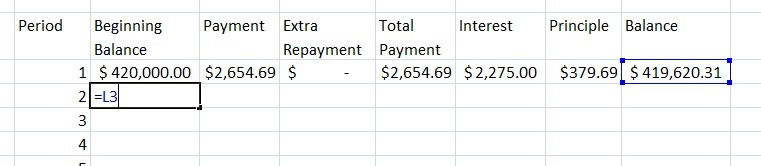
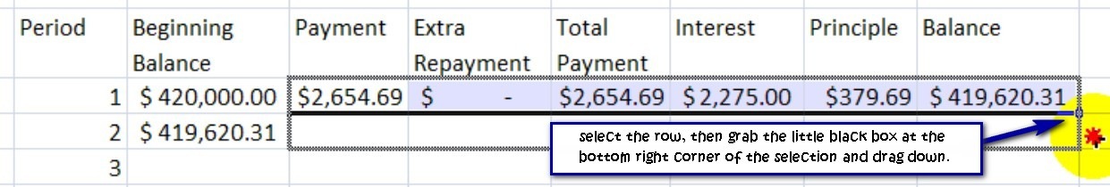
Row two is slightly different. The beginning balance is the same as last months ending balance, so put a formula in to point to L3. As we want this formula to change as we fill down the rest of the table, we’re not going to lock it in as an absolute reference.

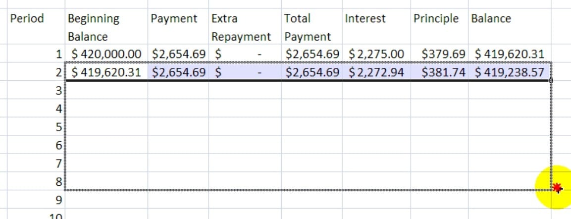
The rest of the row can be copied down by selecting across the row from payment amount to balance and grabbing our fill handle and dragging down. Have a look at the formulae in row 2 by double clicking. You should find that the absolute references still point to our initial data, but the rest of the formulae have changed appropriate for row two. The ending balance has also reduced by the principle portion of our payment.

Now fill the rest of the table all the way down to period 360 by selecting all of row 2 from beginning balance to end balance and filling down using our fill button.

You should find that at the bottom of the table, after the last (360th) monthly payment, the end balance is $0.

Using Excel to Run Different Loan Repayment Scenarios

All results are based on the assumption that the interest rate remains fixed throughout the entire loan term and that interest is calculated monthly and payments made monthly. It does not take into account bank fees. Note that banks can often have their own confusing way of calculating interest!

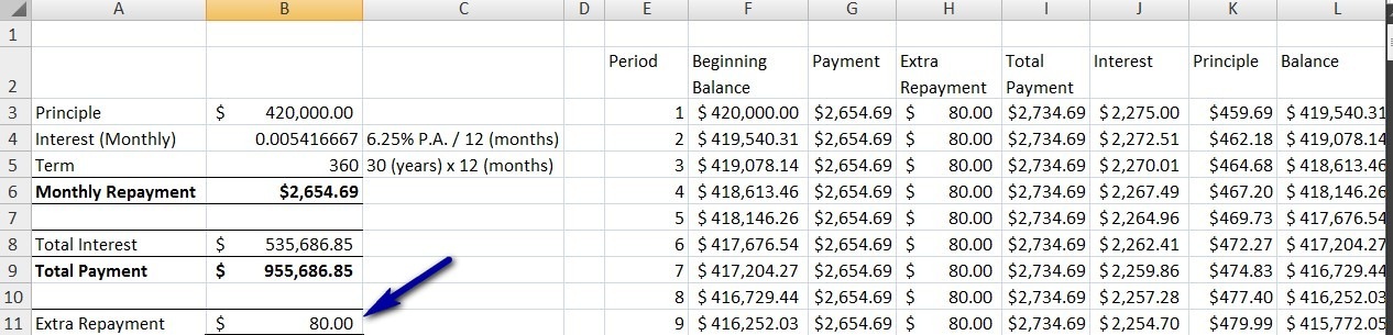
Continuing on, let’s start by putting in our extra repayment amount. We will put this in the field under our PMT data, and make it $80 per month. Because we’ve already formatted our table, the extra repayment column updates automatically as well as all the other cells in the table.

Of course, when we make extra repayments, we’re paying our loan off quicker, so if you scroll to the bottom of the table you will notice that there are negative numbers for the rest of the loan term after the ending balance equals $0. We are going to edit the formulae that we created in Part One to include if statements, so that when our loan balance comes to $0, the calculations automatically end. That way we will be able to summarise the information in our results table.

First, in order to stop the period counting down once the balance has reached $0, we will adjust the formula from period 2 down to the following:

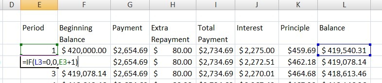
The calculation basically says that if the ending balance of my last payment period equals $0, then the number in the period column equals zero, otherwise, take the above period number and add one. Double click on the fill handle to fill down the entire table. Nothing will change just yet, the period should still count from 1 to 360, but once we start changing the other formulae, you will see this column change.

Next, we will add an if statement to the payment column starting at row 2 as per the following:

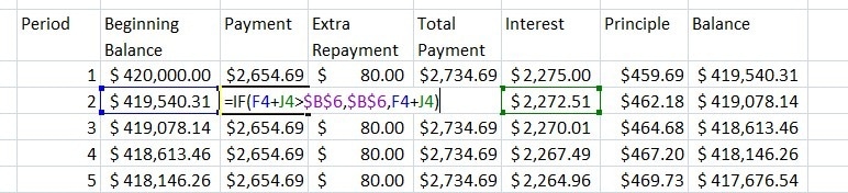
This calculation says that if the monthly payment amount (at B6) is more than the beginning balance for the period (F4) plus the interest amount (J4), then show the monthly payment amount, otherwise (if the beginning balance plus the interest is less than the monthly payment amount) calculate the monthly payment amount as the balance plus interest. Once you’ve typed the formula, use the fill handle to fill down the column.

Finally, we will add a similar if statement to the extra repayment starting at row 2 as follows and fill down as before:

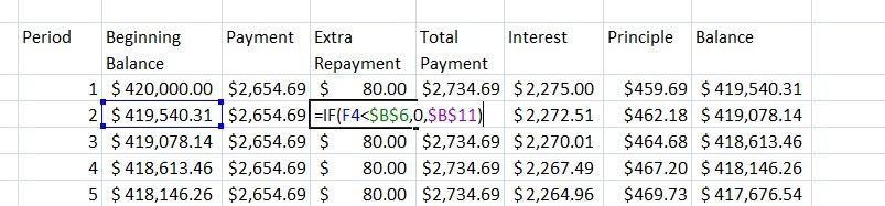
So, if the balance at the beginning of the month is less than the monthly payment amount (B6) then make $0 extra repayment, otherwise, use the extra repayment amount as we set up in B11. You will notice that for these two formulae, we have used the dollar signs for absolute references to lock in the numbers from our data table for when we fill down.

Have a look towards the bottom of the spreadsheet and you will notice that with the extra repayment of $80 per month, we will have paid off our loan 30 months early (period 331). Everything after that has been changed from negative numbers to zeros.

Now we can leave our amortisation table as is and it is just fine, or we can use some conditional formatting to hide any 0 amounts and make it look pretty. The conditional formatting will mean that any cell that has a 0 in it will be “hidden” and the hidden cells will change automatically if we change our extra repayment amount.

Select the entire table range from E3 to L362, open up the conditional formatting dialogue from the Home ribbon and select New Rule. Click on the option use formula to determine which cells to format and enter the following formula:

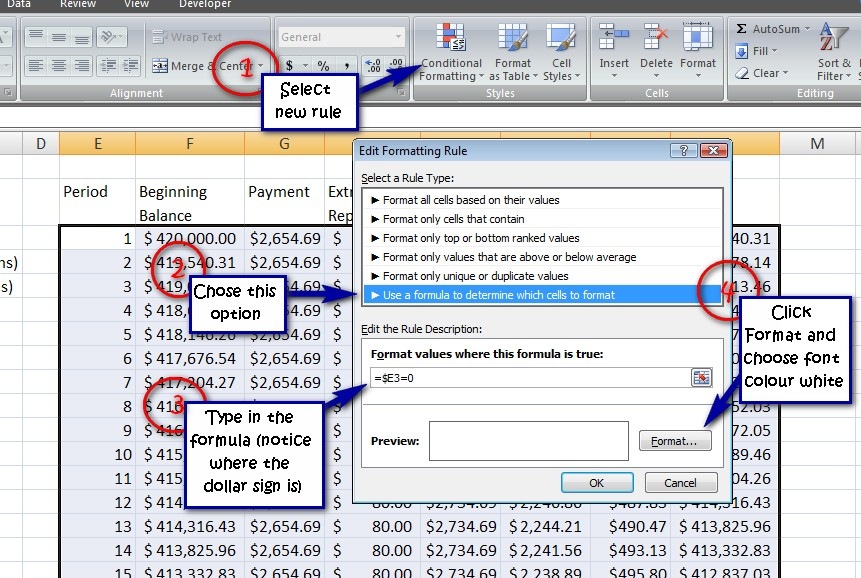
What this formula is saying is that if there is a 0 in the cells in column E, then format the text to white so we can’t see it. It’s still there, just not visible. Have a look at the bottom of the table. It should now look like it ends at period 331 with the final ending balance being $0.

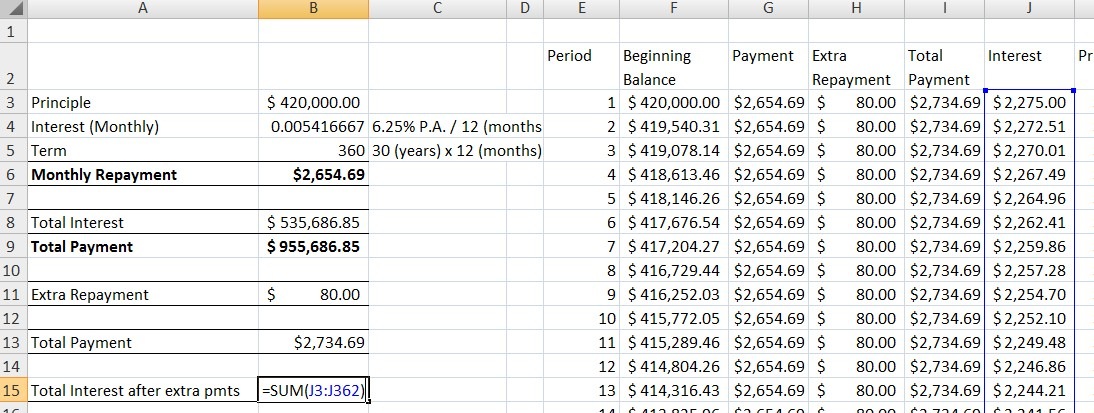
Over to the left of our table, well put in some fields to summarise some key results. Add a heading to show total interest paid (as per the table once extra repayments are taken into account), and use the auto sum formula to add up all of the monthly interest amounts. Make sure that you select all the way down to row 362 to include all of the hidden cells.

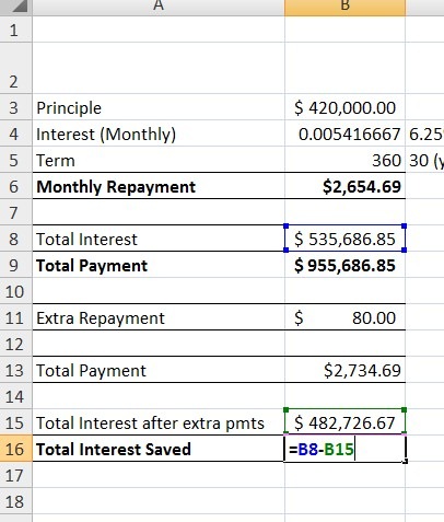
Subtract the total interest after extra pmts from the total interest as per our CUMIPMT calculation in B8 to find out how much interest you save by making extra repayments.

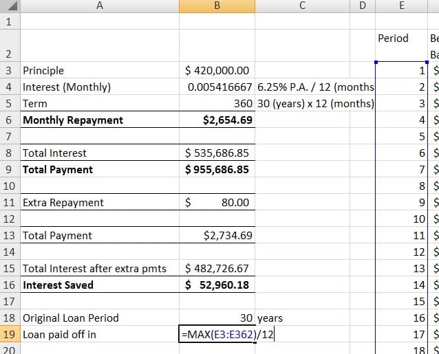
Beneath this, we will use the max function divided by 12 to work out the time in years that it will take to pay off the loan when making extra repayments and how many years and months we shaved off the loan term. Remember to select the range E3 all the way to E362 to include the hidden data.

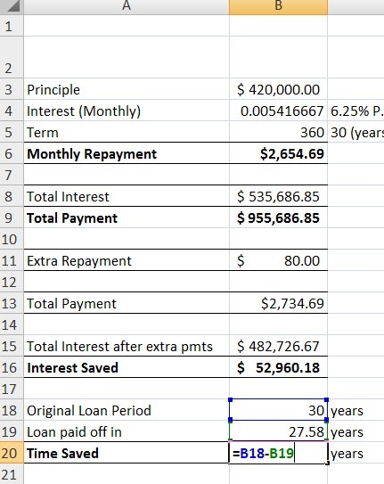
If necessary, format these cells as ‘number’ and reduce the number of decimal places.

Add a heading, pretty it up with some formatting to make it easier to read. I’ve rearranged some of the data in the tables to organise it a bit better, your final product might look something like this:

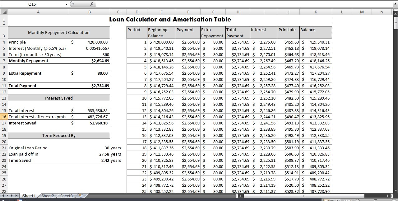
That’s it! Now we can run some scenarios by changing the variables under the monthly repayment calculations such as the interest rate, the extra repayment amount or the principal amount. Because everything is formulated, changing one variable will mean that the entire amortisation table will adjust automatically and the interest saved and loan period will also be adjusted automatically and that’s the exciting part about Excel! And once you have this spreadsheet set up, you can copy and paste it into multiple sheets and use it to calculate other loans like a car loan.

Have a go changing the extra repayment amount to $120. How much interest do you save? How much time? What about if the interest rate is 7%? What is the repayment amount?

Linking Our Repayment Report with our Budget to See How Various Scenarios affect Our Cash Flow

All results are based on the assumption that the interest rate remains fixed throughout the entire loan term and that interest is calculated monthly and payments made monthly. It does not take into account bank fees. Banks often have their own confusing ways of calculating interest, so your results may differ from theirs.

Below is an example of a cash flow budget. You will notice it’s incomplete but it gives us an idea of how this works. I’ve previously written a post on how to set a cash flow budget, but not specifically how to do it in excel, so if you would like me to write a tutorial on that, let me know.

I just pulled the numbers in the cash flow budget off the top of my head and they don’t reflect any real-life information.

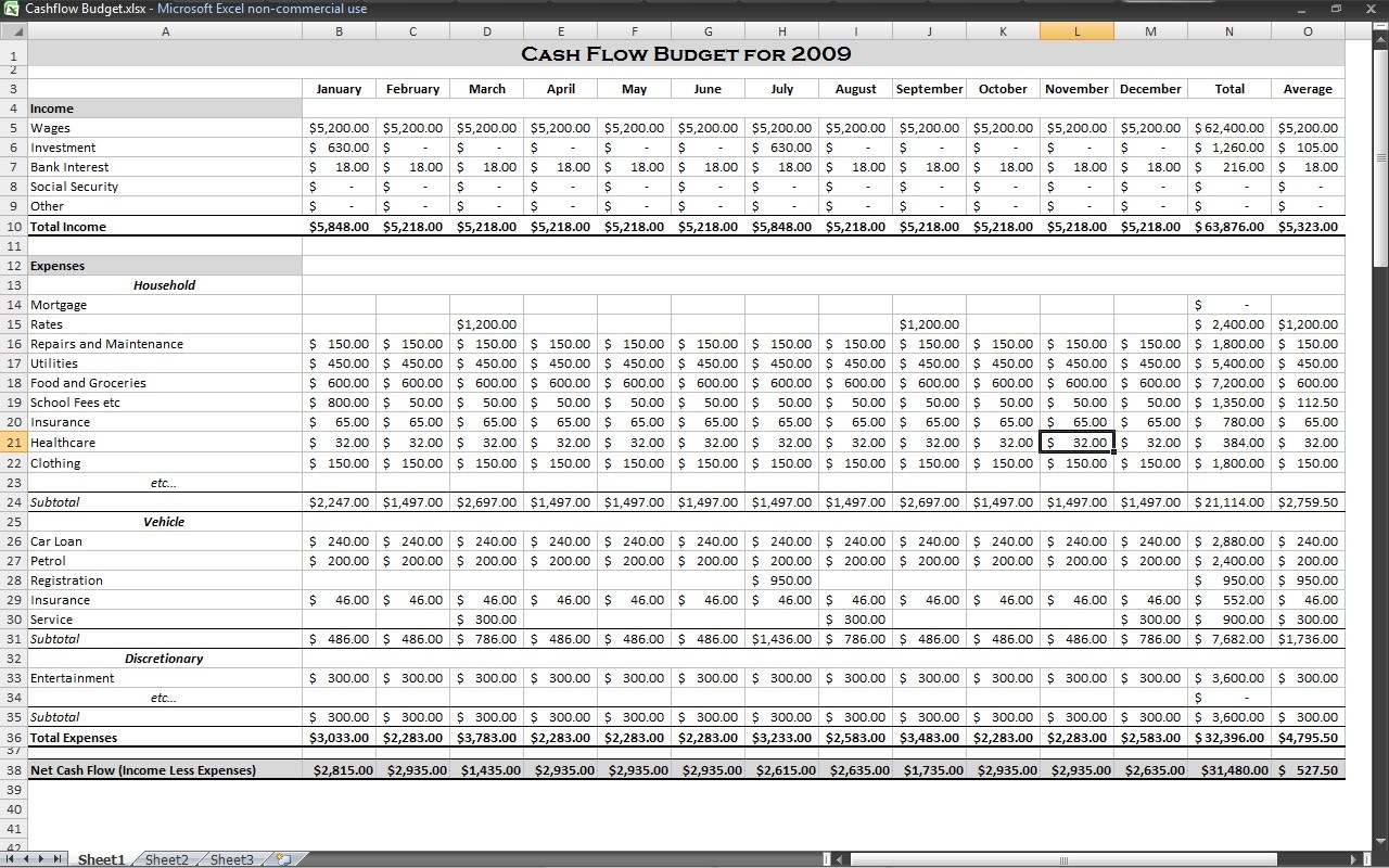
You will notice that I’ve left the mortgage field in the spreadsheet blank, this is where we will put in our linking formula.

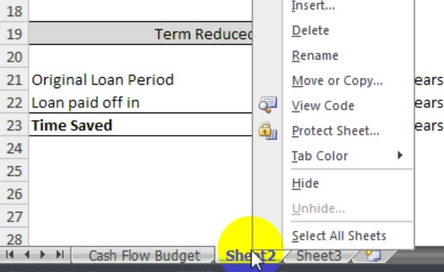
Start by renaming Sheet 1 to Cash Flow Budget by right-clicking on the tab and selecting Rename. If you have already created a loan calculator and amortisation table, copy and paste the entire sheet into Sheet 2 and rename Sheet 2 Loan Calc.

Now in the first mortgage cell under January in our cash flow budget (B13) we are going to enter a reference formula:

1. Type = (equals)

2. Click on the Loan Calc tab

3. Click on the total payment amount in our left-hand data table (B11 on my sheet)

4. Press F4 on the keyboard to make the reference absolute (2 dollar signs will appear in the formula).

5. Press Enter

The formula will look like this:

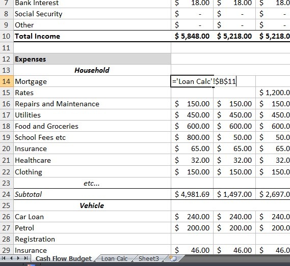
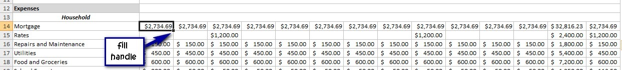
This will bring across our monthly mortgage payment amount from our loan calculations spreadsheet. Now just grab the fill handle at the bottom and drag to fill across to December. If you double-click on any of the cells along this row, you will notice that the formula points back to the monthly payment cell on the Loan Calculations page.

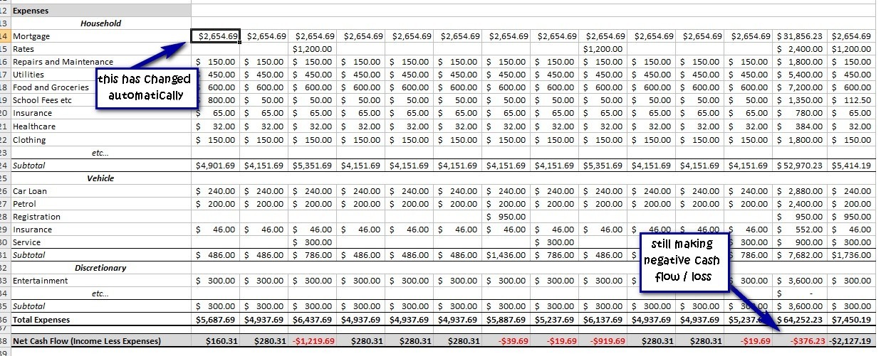
Adding the mortgage repayment into you Cash Flow Budget will automatically change the totals for Total Expenses and Net Cash Flow. In the spreadsheet that I created, once we put in the mortgage repayments, we end up with a negative cash flow balance, so it would seem that we can’t afford a $420,000 loan.

So I’m going to go back to our loan calculation sheet and change the extra repayment amount to $0 and have a look at the effect on our cash flow. You will notice that the amortisation table and the results data change automatically and we will now not be saving any money on interest or reducing the loan term.

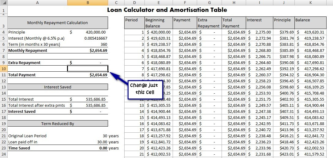
My cash flow budget will also automatically update just by changing the data in this one cell, but it looks like I still can’t afford the loan repayment.

So back on my loan calc sheet, I’ll change the principle (the amount we are thinking of borrowing) to $400,000 and make extra repayments of $50 per month.

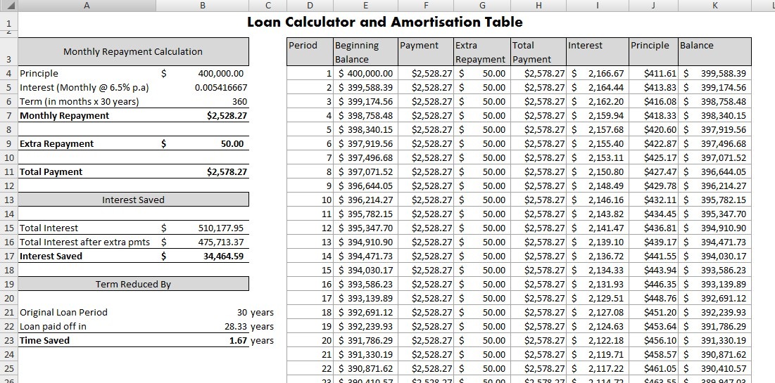
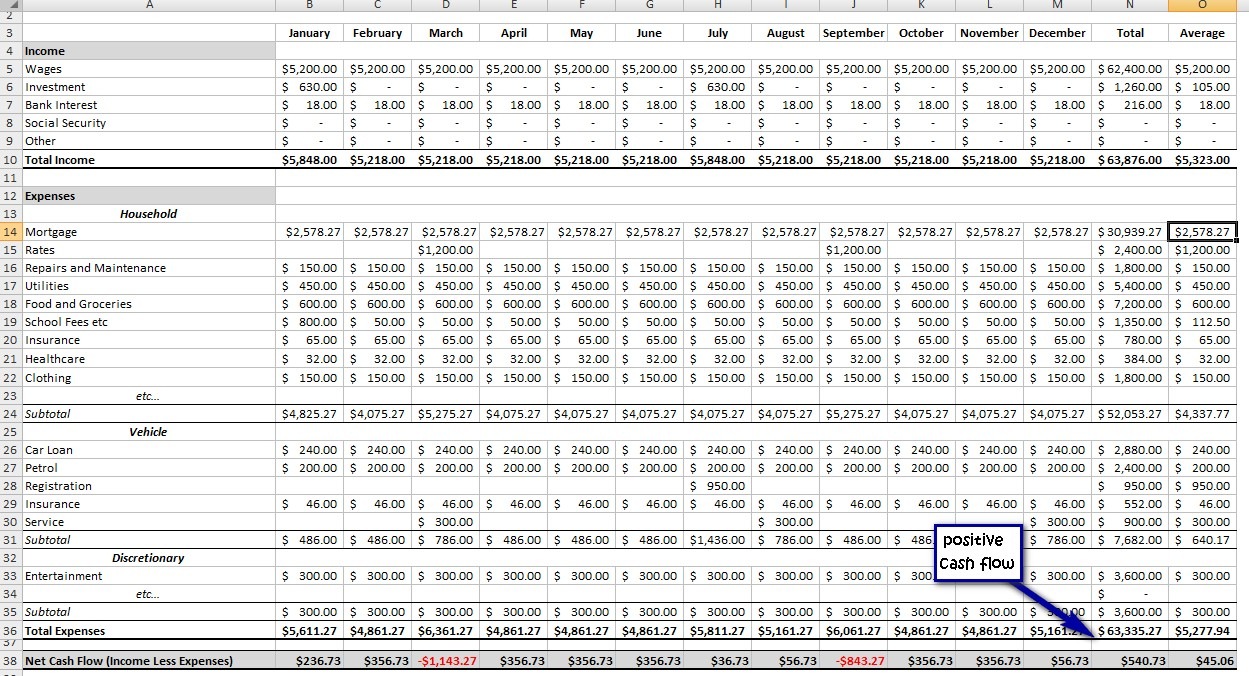
By changing the principal amount I can instantly see that I can afford to make the loan repayments. I can also see that I’m saving around $34,000 in interest and shaving 1.67 years off the loan by making extra repayments.

You will also see the effects on your cash flow if you change the interest rate or reduce the term of the loan making your spreadsheet a pretty powerful personal financial forecaster! Huge companies like BHP use similar techniques (just more sophisticated) for their financial modelling with exactly the same software that we use at home.

We created this loan calculator just for a mortgage, but you can copy and paste your loan calculator onto as many sheets as you need and just change the variables for car repayments or credit card repayments. Use the same formula as above to link these repayments into your cash flow budget.